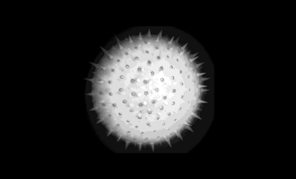
Moving an objective or specimen is not the only way to scan through focal planes. Electrically tunable lenses can shift focus optically, enabling fast axial scanning without translating the objective, sample or a conventional lens group. This guide examines how the approach works in widefield, confocal, two-photon and inspection microscopy—and the system-level trade-offs engineers must consider when integrating it.
Modern microscopy systems are increasingly expected to acquire larger datasets in less time. Whether imaging live biological processes, scanning thick samples, building 3D image stacks, or performing automated inspection, rapid movement through different focal planes has become an important capability. As requirements for acquisition speed and throughput continue to grow, engineers are increasingly evaluating alternatives to traditional mechanically actuated focusing approaches.
In a conventional microscope, changing the focal plane is a mechanical operation. Either the specimen moves on a z-stage, the objective moves relative to the specimen, or a piezo-actuated mount produces a smaller and faster displacement. These approaches are well established, but they all ask a physical assembly to travel along the optical axis.
That becomes consequential when a system must refocus rapidly, repeatedly or across several planes. Mechanical travel introduces inertia, consumes space and can affect settling time, lifetime and system architecture. In applications involving dynamic biological processes, rapid volumetric imaging or high-throughput inspection, the focusing mechanism can become one of the factors limiting acquisition speed.
A focus-tunable lens changes the problem. Instead of translating the sample or objective, it changes the convergence or divergence of the beam entering the objective. The focal plane moves, while the objective and specimen remain stationary.
Depending on the optical design, performance requirements and implementation, electrically tunable lenses can provide axial focusing ranges from approximately 30 to 700 micrometres in microscopy systems. In one demonstrated configuration, a 100-micrometre focus shift was achieved in 15 milliseconds with a 40x, NA 0.8 objective.
Those figures are compelling, but they do not mean that a tunable lens can simply be added anywhere in the optical path. Its position affects telecentricity, magnification, field of view, numerical aperture and the complexity of the surrounding optics. The most successful implementation begins by treating the tunable lens as part of the complete optical system—not as an isolated replacement for a translation stage.
How optical focusing works in an infinity-corrected microscope
Most modern microscope objectives are infinity corrected. Light originating from a point in the nominal focal plane leaves the objective as a collimated beam. A separate tube lens then forms the image on the detector.
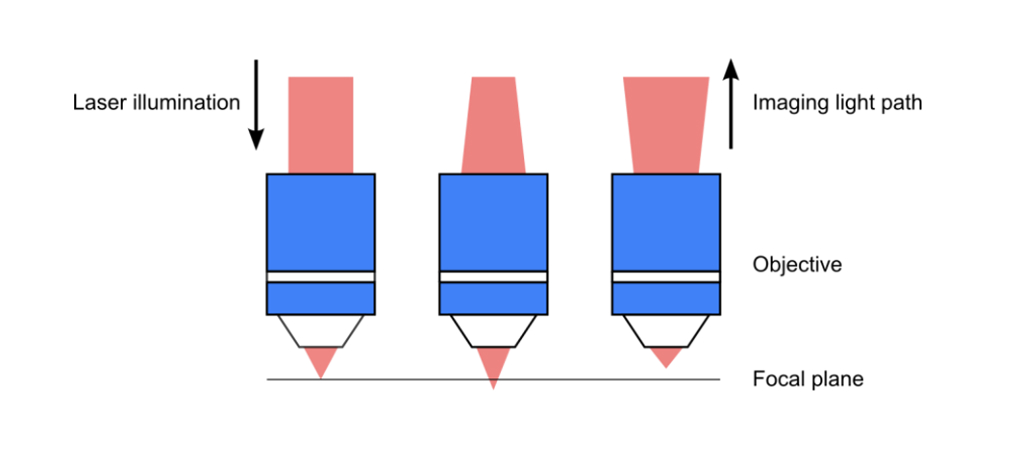
If the object lies closer to the objective than the nominal working distance, the emerging beam diverges. If the object lies farther away, the beam converges. The same relationship can be used in reverse: changing the curvature of the beam presented to the objective changes the axial position at which the objective focuses.
An electrically tunable lens, or ETL, creates that variable wavefront curvature. The focal power of the lens changes with the applied current, allowing the microscope to refocus electronically. When a system must tune across both converging and diverging conditions, the ETL can be paired with a negative offset lens. In the configuration evaluated by Optotune, an EL-10-30 was combined with a plano-concave offset lens with a focal length of -100 mm.
This ETL and offset-lens assembly can be mounted in a custom holder or standard lens tube. Its physical integration can therefore be relatively simple. Its optical location requires more careful consideration.
Where should the tunable lens be positioned?
There are two principal approaches: placing the ETL assembly close to the objective, or placing it at a plane conjugate to the objective pupil.
Option 1: Close to the objective
The most straightforward arrangement is to position the ETL and offset lens near the rear of the objective. The assembly may be inserted between the objective turret and objective, in much the same location as a piezoelectric focusing device.
In one model using a 40x objective with a 4.4 mm focal length, changing the ETL focal length from 150 to 80 mm shifted the axial focus from approximately -50 to +50 micrometres around the nominal working distance. The complete assembly had an axial length of about 50 mm.
The simplicity comes with a trade-off. Placing the tunable lens close to the objective generally creates non-telecentric conditions. As the axial focal position changes, the magnification and field of view can change as well. The effective numerical aperture—and therefore resolution—may also vary across the focusing range.
For relatively small focus shifts, typically below about 50 micrometres, these effects may be tolerable. This approach can also work well in applications where a modest change in field size does not interfere with the measurement.
Option 2: At a conjugate pupil plane
When stable magnification is important, the ETL assembly can instead be positioned at a plane conjugate to the objective pupil. Because the pupil of a microscope objective is usually inaccessible, a 4f relay system can be used to reproduce it at a convenient location.
Placing the ETL at this conjugate plane preserves telecentric imaging and avoids the change in field of view or magnification associated with the near-objective configuration. It is therefore preferable for visual microscopy and other applications in which apparent zoom during focusing would be distracting or analytically unacceptable.
The cost is additional optical and mechanical complexity. A relay system requires space, careful alignment and suitable access to the microscope’s light path. Depending on the beam size and operating conditions, vignetting at the objective front lens can also change the effective numerical aperture.
There is no universally correct integration strategy. The optimal location depends on the microscope architecture, required focus range, acceptable image variation, and available optical and mechanical space.
| Integration approach | Principal advantage | Principal limitation | Typical fit |
|---|---|---|---|
| ETL close to the objective | Compact and comparatively straightforward | Magnification, field of view and numerical aperture may change with focus | Small focusing ranges, confocal and two-photon configurations where the change is acceptable |
| ETL at a conjugate pupil | Preserves magnification and field of view across the focusing range | Requires relay optics, alignment and physical space | Custom microscopes, visual use and applications requiring telecentric behaviour |
Widefield microscopy: preserving the field while moving the focal plane
In visual and widefield microscopy, a change in magnification during focusing appears as a zoom. Small shifts of a few micrometres may be acceptable; larger changes are likely to be distracting and can complicate quantitative imaging.
For this reason, a conjugate-pupil implementation is generally the stronger option. In an inverted microscope, the internal optics may already create an accessible conjugate pupil. If not, a relay module can reproduce the pupil externally.
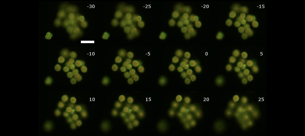
In the Optotune evaluation, an ETL and offset lens were positioned near an accessible pupil in a Zeiss Axiovert 35. With a 40x, NA 0.6 objective, the system achieved a defocusing range of up to 120 micrometres. A fluorescence z-stack of pollen grains was acquired across focal positions from -30 to +25 micrometres without a change in magnification.
The result illustrates the central benefit of pupil-plane placement: the focal plane can move electronically while the image geometry remains stable.
Confocal microscopy: integration inside a tightly packaged system
Confocal microscopes present a different challenge. They are often highly integrated, with limited access to the internal optical path. The theoretical location of an ETL may therefore be less important than the locations that are physically available.
Several configurations are possible:
- The ETL assembly can be placed between the objective and turret.
- It can be integrated into a custom filter cube when that part of the optical path is available during confocal imaging.
- A relay system can be inserted between the confocal scanning unit and microscope stand.
Optotune tested the filter-cube approach in a spinning-disk confocal microscope built around a Yokogawa CSU-X1 unit and an Olympus IX-71 stand. The ETL and offset lens were mounted in a modified filter cube and inserted below the objective turret. Rotating the turret to an empty position removed the assembly from the optical path when it was not required.
With a 40x, NA 1.3 objective, the setup produced a 60-micrometre z-range and was used to acquire a confocal stack through a pollen grain approximately 100 micrometres in diameter.
This example is useful because it shows that ETL integration does not always require rebuilding the microscope. Existing mechanical features can sometimes provide an effective insertion point, although the resulting changes in magnification and numerical aperture still need to be evaluated.
Two-photon microscopy: a particularly strong fit for tunable focusing
Two-photon excitation microscopy is well suited to imaging in scattering tissue. It is widely used, for example, to record neuronal activity at different depths in living brain tissue. Because neurons occupy a volume rather than a single plane, rapid axial access is valuable: sampling one focal plane captures only part of the activity in the local network.
Several characteristics make ETL-based focusing particularly compatible with two-photon systems.
First, axial scanning can often be performed in the excitation path alone. The nonlinear excitation process confines fluorescence generation to the focal region, so changing the excitation focus is sufficient to move the imaging plane.
Second, the near-infrared excitation wavelength makes the system more tolerant of certain wavefront errors than visible-light imaging. The evaluated microscope operated at 850 nm. Its approximately 10 nm spectral bandwidth also limited the effect of chromatic aberrations introduced by the non-achromatic ETL and offset-lens combination.
Third, many functional measurements repeatedly address selected cells rather than relying on perfectly invariant image geometry across every plane. A change in field size may therefore be manageable: the scan positions can be adjusted to address the same cells at different depths.
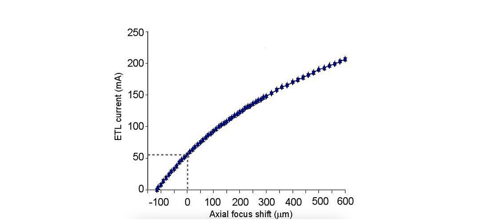
In a custom two-photon microscope, Optotune mounted the ETL and offset lens in an objective holder used with a 40x, NA 0.8 water-immersion objective. Tuning the ETL from 50 to 200 mm focal length produced an axial focusing range of up to 700 micrometres. The objective’s nominal working distance was 3.3 mm, with the demonstrated tuning corresponding to working distances from approximately 2.8 to 3.41 mm.
Most applications do not require the full range. The more important result is that the focal plane can be repositioned quickly and under electronic control. In this setup, a 100-micrometre focus change was demonstrated in 15 milliseconds.
The system must still be calibrated. A lookup table relating drive current to axial focus position provides a practical method for commanding the desired depth. For higher-accuracy or changing environmental conditions, the calibration and control strategy may need to account for the behaviour of the complete optical system.
Light-sheet microscopy and rapid volumetric imaging
The same ability to change focus without translating the objective has relevance in light-sheet microscopy, where acquisition speed and access to three-dimensional samples are central design considerations. Published work using Optotune technology has demonstrated rapid 3D light-sheet microscopy with a tunable lens.
The implementation depends on whether the tunable element is used in the illumination path, detection path or a coordinated optical architecture. The same ability to change focus without moving the objective is also relevant in light-sheet microscopy, where rapid volumetric imaging is often a key requirement. Because light-sheet systems can use tunable optics in different parts of the optical architecture, integration strategies vary depending on the specific design.
Inspection microscopy: electronic focus in a modular optical stack
The principle also extends beyond biological microscopy. In an inspection microscope assembled from standard optical components, the tunable lens can be positioned between an infinity-corrected objective and the tube lens.
Optotune evaluated an off-the-shelf arrangement combining an EL-10-30-Ci with Optem micro-inspection optics and a C-mount camera. The shared C-mount interfaces allowed the components to be combined into a compact stack. As magnification increased, the achievable z-range, depth of field and horizontal field of view decreased, while axial resolution improved.
This relationship is typical of inspection systems: the required field of view, magnification, working distance and axial resolution must be considered together. A tunable lens adds fast electronic focusing, but it does not remove the fundamental optical trade-offs created by numerical aperture and magnification.
Control and calibration
An electrically tunable lens is controlled by adjusting drive current. In the evaluated systems, the EL-10-30 was driven by a precision constant-current source with a programmable output from 0 to 250 mA.
For straightforward focusing tasks, a calibrated lookup table can relate commanded current to axial position. Building that table requires measuring the focal position across the intended operating range in the actual microscope configuration. The relationship should not be treated as a property of the ETL alone: the objective, offset lens, relay optics and alignment all influence the resulting axial displacement.
The required control strategy depends on the application. A system that switches between a small number of predefined planes may use a simple calibration table. A measurement system requiring repeatable absolute positioning across temperature and time may need more extensive characterization or closed-loop feedback.
Integration checklist for focus-tunable microscopy
Before selecting a lens or finalizing the optical layout, consider the following questions.
1. Where can the ETL be inserted?
Identify the accessible optical planes and available mechanical space. In a commercial microscope, the most theoretically desirable plane may not be physically accessible.
2. Must magnification remain constant?
If a change in field of view is unacceptable, position the ETL at a conjugate pupil using existing internal optics or a relay system.
3. What aperture must the system support?
The beam diameter, including the diameter at a conjugate pupil, must fit within the clear aperture of the selected tunable lens. The evaluated EL-10-30 has a 10 mm aperture.
4. What axial range is genuinely required?
With medium- and high-NA objectives, ETLs are particularly well suited to focus ranges from tens to hundreds of micrometres. Low-magnification, low-NA objectives may support larger ranges. For coarse travel, ETL focusing can be combined with a mechanical stage.
5. Which optical properties must remain stable?
Consider field of view, magnification, numerical aperture, resolution, chromatic aberration and wavefront quality across the full tuning range. Simulating the complete microscope is often the most reliable way to understand these interactions.
6. How fast must the system refocus?
Define both the required focus displacement and acceptable settling behaviour. The demonstrated 100-micrometre shift in 15 milliseconds provides a useful reference, but performance must be evaluated in the intended optical and control configuration.
7. How will the system be calibrated?
Decide whether a lookup table is sufficient or whether the application requires temperature compensation, periodic recalibration or feedback from the imaging system.
Choosing between optical and mechanical focusing
Focus-tunable and mechanical focusing should not be treated as mutually exclusive technologies. A mechanical stage remains useful for coarse positioning, long travel and applications in which moving the specimen or objective introduces no meaningful limitation. An ETL is especially valuable when the system requires fast, frequent and programmable movement across a smaller axial range.
Many practical systems can use both: mechanical motion establishes the coarse working position, while the tunable lens performs rapid fine focusing or switches between selected planes.
The decision is therefore not simply whether an ETL is faster. It is whether optical focusing produces a better system once telecentricity, aberrations, aperture, calibration, control and physical integration are considered together.
From moving hardware to controlling the wavefront
The most important change introduced by a focus-tunable lens is architectural. Axial focusing no longer has to mean translating an objective, specimen or lens assembly. It can become an electronically controlled optical function.
In widefield microscopy, that can mean moving through a fluorescence sample while preserving magnification through pupil-plane integration. In confocal systems, it can mean adapting a tightly packaged microscope through an accessible filter position. In two-photon microscopy, it can enable rapid access to neuronal populations at different depths. In inspection, it can add programmable focus to a compact modular optical stack.
The benefits are real, but so are the design choices. The position of the lens, the structure of the relay optics, the required tuning range and the acceptable image variation all determine whether the integration succeeds.
For engineers evaluating focus-tunable microscopy, the right starting question is not simply, “How far can the lens refocus?” It is, “What must remain unchanged while the focal plane moves?”